Difference between revisions of "Lecture 4. - Assignment"
(→Analysis of Cable Parasitics (ANSYS 2D Extractor)) |
|||
| (25 intermediate revisions by the same user not shown) | |||
| Line 14: | Line 14: | ||
| width=50% | | | width=50% | | ||
'''Instructor''' | '''Instructor''' | ||
| − | * Dániel Marcsa (lecturer) | + | * [http://wiki.maxwell.sze.hu/index.php/Marcsa Dániel Marcsa] (lecturer) |
* Lectures: Monday, 14:50 - 16:25 (D201), 16:30 - 17:15 (D105) | * Lectures: Monday, 14:50 - 16:25 (D201), 16:30 - 17:15 (D105) | ||
* Office hours: by request | * Office hours: by request | ||
| Line 22: | Line 22: | ||
* Office hours: -. | * Office hours: -. | ||
|} | |} | ||
| − | + | <blockquote> | |
=== Purpose of the Assignment === | === Purpose of the Assignment === | ||
[[File:Lecture4 ProblemGeometry.png|510px|thumb|right|alt=The geometry of the problem with the yellow cable harness. | The geometry of the problem with the yellow cable harness.]] | [[File:Lecture4 ProblemGeometry.png|510px|thumb|right|alt=The geometry of the problem with the yellow cable harness. | The geometry of the problem with the yellow cable harness.]] | ||
| Line 36: | Line 36: | ||
After launching ANSYS Electronics Desktop, open the file '''CableHarness_Example.aedt''' using the ''File <math> \to </math> Open'' menu. <br/> | After launching ANSYS Electronics Desktop, open the file '''CableHarness_Example.aedt''' using the ''File <math> \to </math> Open'' menu. <br/> | ||
To use [https://www.ansys.com/products/electronics/ansys-q3d-extractor ANSYS 2D Extractor], [https://www.ansys.com/products/electronics/ansys-hfss ANSYS HFSS] and [https://www.ansys.com/products/electronics/ansys-electronics-desktop ANSYS Circuit], the ''Help'' menu and ''YouTube'' videos provide a lot of help. | To use [https://www.ansys.com/products/electronics/ansys-q3d-extractor ANSYS 2D Extractor], [https://www.ansys.com/products/electronics/ansys-hfss ANSYS HFSS] and [https://www.ansys.com/products/electronics/ansys-electronics-desktop ANSYS Circuit], the ''Help'' menu and ''YouTube'' videos provide a lot of help. | ||
| − | + | </blockquote> | |
| − | == | + | == Problem Definition and Results == |
| − | [[File:Cable Evectors.gif|360px|thumb|right|alt=Electric field intensity vectors in the dielectric material. |Electric field intensity vectors in the dielectric material <span style="color:blue">[Click to see animation.]</span> | + | <blockquote> |
| − | + | [[File:Cable Evectors.gif|360px|thumb|right|alt=Electric field intensity vectors in the dielectric material in ''ANSYS 2D Extractor''. |Electric field intensity vectors in the dielectric material in ''ANSYS 2D Extractor'' <span style="color:blue">[Click to see animation.]</span>.]] | |
| − | [[File: | + | [[File:CableHarness Circuit.png|360px|thumb|right|alt=The driving circuit of cable in ''ANSYS Circuit''. | The driving circuit of cable in ''ANSYS Circuit''.]] |
| − | |||
In this case, the whole problem is pre-defined. The reason for this is to avoid lengthy setup and basically, the purpose of the example is to look at the effect of high-frequency cables for the car body. Thanks to this example, students explain why you need to pay attention to the proper cable routing in vehicles. However, we review the structure of this task. | In this case, the whole problem is pre-defined. The reason for this is to avoid lengthy setup and basically, the purpose of the example is to look at the effect of high-frequency cables for the car body. Thanks to this example, students explain why you need to pay attention to the proper cable routing in vehicles. However, we review the structure of this task. | ||
The problem is split into three parts: | The problem is split into three parts: | ||
| − | + | * The analysis of cable (''ANSYS 2D Extractor''); | |
| − | + | * the set up of cable harness electric circuit (''ANSYS Circuit''); | |
| − | + | * and the high-frequency analysis of the car body with cable harness (''ANSYS HFSS''). | |
Before and during the run, we briefly review the settings of the problem. | Before and during the run, we briefly review the settings of the problem. | ||
| Line 54: | Line 53: | ||
=== Analysis of Cable Parasitics (''ANSYS 2D Extractor'') === | === Analysis of Cable Parasitics (''ANSYS 2D Extractor'') === | ||
| + | |||
ANSYS 2D Extractor efficiently performs the 2D quasi-static electromagnetic field simulations (''ANSYS Q3D Extractor for 3D problems'') required for the extraction of RLCG parameters (''R'' - resistance, ''L'' - inductance, ''C'' - capacitance, ''G'' - conductance) from an interconnect structure. | ANSYS 2D Extractor efficiently performs the 2D quasi-static electromagnetic field simulations (''ANSYS Q3D Extractor for 3D problems'') required for the extraction of RLCG parameters (''R'' - resistance, ''L'' - inductance, ''C'' - capacitance, ''G'' - conductance) from an interconnect structure. | ||
| Line 60: | Line 60: | ||
The simulation frequency is 300 MHz and the result of the analysis is shown in the following tables. | The simulation frequency is 300 MHz and the result of the analysis is shown in the following tables. | ||
| − | {| width= | + | {| width=60% |
|- | |- | ||
| align=center | | | align=center | | ||
| − | {| class = "wikitable" style = "text-align: center; width: | + | {| class = "wikitable" style = "text-align: center; width: 300px; height: 100px;" |
|+ Conductance matrix of cable. | |+ Conductance matrix of cable. | ||
! Conductance [<math>\mu\text{S}</math>] | ! Conductance [<math>\mu\text{S}</math>] | ||
| Line 77: | Line 77: | ||
|} | |} | ||
| align=center | | | align=center | | ||
| − | {| class = "wikitable" style = "text-align: center; width: | + | {| class = "wikitable" style = "text-align: center; width: 300px; height: 100px;" |
|+ Capacitance matrix of cable. | |+ Capacitance matrix of cable. | ||
! Capacitance [<math>\mu\text{F}</math>] | ! Capacitance [<math>\mu\text{F}</math>] | ||
| Line 92: | Line 92: | ||
|- | |- | ||
| align=center | | | align=center | | ||
| − | {| class = "wikitable" style = "text-align: center; width: | + | {| class = "wikitable" style = "text-align: center; width: 300px; height: 100px;" |
|+ Resistance matrix of cable. | |+ Resistance matrix of cable. | ||
! Resistance [<math>\Omega</math>] | ! Resistance [<math>\Omega</math>] | ||
| Line 106: | Line 106: | ||
|} | |} | ||
| align=center | | | align=center | | ||
| − | {| class = "wikitable" style = "text-align: center; width: | + | {| class = "wikitable" style = "text-align: center; width: 300px; height: 100px;" |
|+ Inductance matrix of cable. | |+ Inductance matrix of cable. | ||
! Inductance [<math>\mu\text{H}</math>] | ! Inductance [<math>\mu\text{H}</math>] | ||
| Line 122: | Line 122: | ||
=== Driving Circuit of Cable Harness (''ANSYS Circuit'') === | === Driving Circuit of Cable Harness (''ANSYS Circuit'') === | ||
| + | [[File:CableHarsness EField.gif|510px|thumb|right|alt=The electric field intensity in the wire and in the car body in ''ANSYS HFSS''. | The electric field intensity in the wire and in the car body in ''ANSYS HFSS''. <span style="color:blue">[Click to see animation.]</span>]] | ||
| + | The return path is grounded, while a port with 50<math>\Omega</math> terminal impedance is defined for the negative and positive conductor. The parasitic parameters of the cable veins are coming from the 2D Extractor simulation. The results of this circuit simulation are used as the excitation of finite element simulation in HFSS. | ||
| + | |||
| + | The excitation of the two non-grounded wires of the cable is sinusoidal. The amplitude of sine excitation is 0.5V, and the phase difference between negative and positive wires is 180 degree. | ||
=== Car Body with Cable Harness (''ANSYS HFSS'') === | === Car Body with Cable Harness (''ANSYS HFSS'') === | ||
| − | + | ANSYS HFSS (''High Frequency Structure Simulator'') is a 3D electromagnetic simulation software for designing and simulating high-frequency electronic products such as antennas, radar systems, high-speed electronics found in communications systems (e.g. mobile phone), advanced driver assistance systems (ADAS), satellites, IC packages and internet-of-things (IoT) products. | |
| − | + | ||
| − | + | This example can be regarded as an open problem where the radiation boundary condition is used as a boundary condition. For this problem, we solve the vector wave equation. The car body is taken into account as a finite conductivity boundary and the excitation is the incident field from the cable network. | |
| − | + | As a result, the electric and the magnetic field intensities are visible on the car body. You can see the effect of the cable harness on these animations. | |
| − | + | </blockquote> | |
| − | |||
| − | |||
| − | |||
| − | |||
| − | |||
| − | |||
| − | |||
| − | |||
| − | |||
| − | |||
| − | |||
| − | |||
| − | |||
| − | |||
| − | |||
| − | |||
| − | |||
| − | |||
| − | |||
| − | |||
| − | |||
| − | |||
| − | |||
| − | |||
| − | |||
| − | |||
| − | |||
== References == | == References == | ||
{{reflist}} | {{reflist}} | ||
Latest revision as of 20:52, 28 January 2020
|
Cable Harness Analysis | |
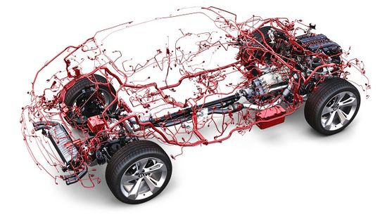
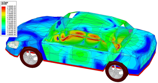
| Whole wiring of a vehicle. | The magnetic field intensity in the wire and in the car body. [Click to see animation.] |
|
Instructor
|
Teaching Assistants:
|
Contents
Purpose of the Assignment
The student will learn the main steps of the finite element method, such as preparing the model (creating or importing geometry), specifying material parameters, boundary conditions, and excitation through a full-wave problem. This example gives a brief insight into the cable harness analysis through an automotive example.
Knowledge needed to solve the problem
- The steps of the finite element method;
- Theoretical knowledge of full-wave fields (for defining materials, excitation);
- Basic knowledge of electric network theory.
Steps to solve the problem
After launching ANSYS Electronics Desktop, open the file CableHarness_Example.aedt using the File [math] \to [/math] Open menu.
To use ANSYS 2D Extractor, ANSYS HFSS and ANSYS Circuit, the Help menu and YouTube videos provide a lot of help.
Problem Definition and Results
In this case, the whole problem is pre-defined. The reason for this is to avoid lengthy setup and basically, the purpose of the example is to look at the effect of high-frequency cables for the car body. Thanks to this example, students explain why you need to pay attention to the proper cable routing in vehicles. However, we review the structure of this task.
The problem is split into three parts:
- The analysis of cable (ANSYS 2D Extractor);
- the set up of cable harness electric circuit (ANSYS Circuit);
- and the high-frequency analysis of the car body with cable harness (ANSYS HFSS).
Before and during the run, we briefly review the settings of the problem.
It is important to note that in the previous two examples, adaptive meshing used. However, in the case of a time-dependent (transient) problem, it is not possible to use the adaptive mesh, so we need to define the discretization of the problem with different mesh operations.
Analysis of Cable Parasitics (ANSYS 2D Extractor)
ANSYS 2D Extractor efficiently performs the 2D quasi-static electromagnetic field simulations (ANSYS Q3D Extractor for 3D problems) required for the extraction of RLCG parameters (R - resistance, L - inductance, C - capacitance, G - conductance) from an interconnect structure.
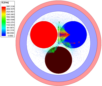
As you can see in the figure, the cable has positive, negative and return veins. The veins wrapped by insulation and the outer sheath.
The simulation frequency is 300 MHz and the result of the analysis is shown in the following tables.
Conductance matrix of cable. Conductance [[math]\mu\text{S}[/math]] Negative Positive Negative 48.46 -24.23 Positive -24.23 48.46
Capacitance matrix of cable. Capacitance [[math]\mu\text{F}[/math]] Negative Positive Negative 117.269 -58.634 Positive -58.634 117.268
Resistance matrix of cable. Resistance [[math]\Omega[/math]] Negative Positive Negative 1.912 0.941 Positive 0.941 1.895
Inductance matrix of cable. Inductance [[math]\mu\text{H}[/math]] Negative Positive Negative 0.134 0.067 Positive 0.067 0.134 Driving Circuit of Cable Harness (ANSYS Circuit)
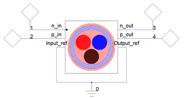
The return path is grounded, while a port with 50[math]\Omega[/math] terminal impedance is defined for the negative and positive conductor. The parasitic parameters of the cable veins are coming from the 2D Extractor simulation. The results of this circuit simulation are used as the excitation of finite element simulation in HFSS.
The excitation of the two non-grounded wires of the cable is sinusoidal. The amplitude of sine excitation is 0.5V, and the phase difference between negative and positive wires is 180 degree.
Car Body with Cable Harness (ANSYS HFSS)
ANSYS HFSS (High Frequency Structure Simulator) is a 3D electromagnetic simulation software for designing and simulating high-frequency electronic products such as antennas, radar systems, high-speed electronics found in communications systems (e.g. mobile phone), advanced driver assistance systems (ADAS), satellites, IC packages and internet-of-things (IoT) products.
This example can be regarded as an open problem where the radiation boundary condition is used as a boundary condition. For this problem, we solve the vector wave equation. The car body is taken into account as a finite conductivity boundary and the excitation is the incident field from the cable network.
As a result, the electric and the magnetic field intensities are visible on the car body. You can see the effect of the cable harness on these animations.


