Difference between revisions of "Lecture 2. - Assignment"
(→Evaluation of results) |
(→Evaluation of results) |
||
| (6 intermediate revisions by the same user not shown) | |||
| Line 14: | Line 14: | ||
| width=50% | | | width=50% | | ||
'''Instructor''' | '''Instructor''' | ||
| − | * Dániel Marcsa (lecturer) | + | * [http://wiki.maxwell.sze.hu/index.php/Marcsa Dániel Marcsa] (lecturer) |
* Lectures: Monday, 14:50 - 16:25 (D201), 16:30 - 17:15 (D105) | * Lectures: Monday, 14:50 - 16:25 (D201), 16:30 - 17:15 (D105) | ||
* Office hours: by request | * Office hours: by request | ||
| Line 22: | Line 22: | ||
* Office hours: -. | * Office hours: -. | ||
|} | |} | ||
| − | + | <blockquote> | |
=== Purpose of the Assignment === | === Purpose of the Assignment === | ||
The student will learn the main steps of the finite element method, such as preparing the model (creating or importing geometry), specifying material parameters, boundary conditions and excitation through a time-harmonic simulation. Give a deeper understanding of the physical background of induction heating, melting and hardening. | The student will learn the main steps of the finite element method, such as preparing the model (creating or importing geometry), specifying material parameters, boundary conditions and excitation through a time-harmonic simulation. Give a deeper understanding of the physical background of induction heating, melting and hardening. | ||
| Line 28: | Line 28: | ||
=== Knowledge needed to solve the problem === | === Knowledge needed to solve the problem === | ||
* The steps of the finite element method; | * The steps of the finite element method; | ||
| − | * Theoretical knowledge of time-harmonic field (for defining materials, for excitation). | + | * Theoretical knowledge of the time-harmonic field (for defining materials, for excitation). |
=== Steps to solve the problem === | === Steps to solve the problem === | ||
After launching ANSYS Electronics Desktop, select ''Project -> Insert Maxwell 3D Design'' from the menu. <br/> It is also possible to solve the problem differently from the steps described below. To use [https://www.ansys.com/products/electronics/ansys-maxwell ANSYS Maxwell], the ''Help'' menu and ''YouTube'' videos provide a lot of help. | After launching ANSYS Electronics Desktop, select ''Project -> Insert Maxwell 3D Design'' from the menu. <br/> It is also possible to solve the problem differently from the steps described below. To use [https://www.ansys.com/products/electronics/ansys-maxwell ANSYS Maxwell], the ''Help'' menu and ''YouTube'' videos provide a lot of help. | ||
| − | + | </blockquote> | |
== Creating Geometry == | == Creating Geometry == | ||
| + | <blockquote> | ||
In this case, we work with a pre-prepared geometry. This corresponds to the design of a geometry that a simulator engineer uses for numerical analysis of the device. | In this case, we work with a pre-prepared geometry. This corresponds to the design of a geometry that a simulator engineer uses for numerical analysis of the device. | ||
So the geometry is imported for this task. The geometry can be imported using the ''Modeler <math>\to</math> Import ...'' menu. | So the geometry is imported for this task. The geometry can be imported using the ''Modeler <math>\to</math> Import ...'' menu. | ||
| − | + | </blockquote> | |
== Problem Settings == | == Problem Settings == | ||
| − | + | <blockquote> | |
=== Defining Materials === | === Defining Materials === | ||
In this exercise, the current carrying coil is ''copper'', the iron is ''cast iron'' and the surrounding region of the coil and iron is ''air''. | In this exercise, the current carrying coil is ''copper'', the iron is ''cast iron'' and the surrounding region of the coil and iron is ''air''. | ||
| Line 71: | Line 72: | ||
I used this mesh on the surface of the cast iron rod, as shown in the figure. From ANSYS Maxwell 2019R1 version, the adaptive mesh does not change the resolution for those areas where ''Skin Depth Based ...'' mesh is defined. The purpose of this is faster convergence, but it is therefore important to define properly the resolution in the penetration depth. | I used this mesh on the surface of the cast iron rod, as shown in the figure. From ANSYS Maxwell 2019R1 version, the adaptive mesh does not change the resolution for those areas where ''Skin Depth Based ...'' mesh is defined. The purpose of this is faster convergence, but it is therefore important to define properly the resolution in the penetration depth. | ||
| + | </blockquote> | ||
| + | == Set up the solver, run the simulation == | ||
| + | <blockquote> | ||
| + | As I wrote in the mesh settings, the adaptive meshing algorithm automatically refines the discretization within the critical regions. However, the adaptive meshing parameters should be set at the solver. The maximum number of adaptive steps (''Maximum Number of Passes'') is 10, and the 'Percent Error' is 0.5%. The refinement rate (''Refinement Per Pass'') should be lowered from the default value (30%) in the case of a three-dimensional problem. This is especially true if we have no prior information on how to converge, how the error is reduced in the example. The refinement rate will be 20%. At the solver, you can specify the frequency of harmonic analysis (''Adaptive Frequency''), in this example <math>f = 500~\text{Hz}</math>. | ||
| − | + | In addition to the previous settings, it is still possible to set the nonlinear residue (''Nonlinear Residual''), but in this example, all materials have linear magnetization curve. If necessary, you can turn on the iterative solver instead of the direct solver, where you also need to define the ''Relative Residual'' as termination criteria. In addition to adaptive mesh refinement, it is possible to use higher order shape functions (''Use higher order shape functions'') for time-harmonic problems and, if necessary, the frequency sweep (''Frequency Sweep'') range and the associated frequency step. | |
| − | + | </blockquote> | |
| − | |||
| − | |||
| − | |||
| − | |||
== Evaluation of results == | == Evaluation of results == | ||
| + | <blockquote> | ||
| + | In addition to the variables (inductance, force) seen in the previous assignments, we can determine the losses in the iron or the coil in this problem. These quantities can also be analysed as a function of frequency (''Frequency Sweep''). | ||
| − | + | [https://www.ansys.com/products/electronics/ansys-maxwell ANSYS Maxwell] automatically calculates losses in the problem, but if we are curious about the eddy current loss in arbitrary part of the problem (e.g. in the cast iron rod), it should be calculated by 'Calculator' (Maxwell 3D <math>\to</math> Fields <math>\to</math> Calculator...). The eddy current loss can be calculated with the following relationship | |
| − | |||
| − | [https://www.ansys.com/products/electronics/ansys-maxwell ANSYS Maxwell] automatically calculates losses in the problem, but if we are curious about the eddy current loss in arbitrary part of the problem (e.g. in the cast iron rod), it should be | ||
::<math> P_{ö} = \frac{1}{2}\int_{V} \vec{J}\cdot\vec{E}^{*}\,\text{d}V = \int_{V} \frac{\vec{J}\cdot\vec{J}^{*}}{2\sigma}\,\text{d}V\quad[\text{W}]</math>. | ::<math> P_{ö} = \frac{1}{2}\int_{V} \vec{J}\cdot\vec{E}^{*}\,\text{d}V = \int_{V} \frac{\vec{J}\cdot\vec{J}^{*}}{2\sigma}\,\text{d}V\quad[\text{W}]</math>. | ||
| Line 93: | Line 94: | ||
* Output <math>\to</math> Eval | * Output <math>\to</math> Eval | ||
| − | The spatial variables can also be plot in various forms, as illustrated by the following two figures. | + | The spatial variables can also be the plot in various forms, as illustrated by the following two figures. |
{| width=100% | {| width=100% | ||
| Line 102: | Line 103: | ||
[[File:InductionHeating OhmicLoss.png|550px]] | [[File:InductionHeating OhmicLoss.png|550px]] | ||
|- | |- | ||
| − | |align=center | <span style="font-size:88%;">'''The streamlines of magnetic field intensity (''ANSYS Maxwell'').</span> | + | |align=center | <span style="font-size:88%;">'''The streamlines of magnetic field intensity (''ANSYS Maxwell'').'''</span> |
| − | |align=center | <span style="font-size:88%;">'''The eddy current loss on the surface of the cast iron rod (''ANSYS Maxwell'').</span> | + | |align=center | <span style="font-size:88%;">'''The eddy current loss on the surface of the cast iron rod (''ANSYS Maxwell'').'''</span> |
|} | |} | ||
| Line 115: | Line 116: | ||
[[File:InductionHeating_OhmicLoss_DiscoveryAIM.png|550px]] | [[File:InductionHeating_OhmicLoss_DiscoveryAIM.png|550px]] | ||
|- | |- | ||
| − | |align=center | <span style="font-size:88%;">'''The magnetic field intensity in the cross-section of the problem (''ANSYS Discovery AIM'').</span> | + | |align=center | <span style="font-size:88%;">'''The magnetic field intensity in the cross-section of the problem (''ANSYS Discovery AIM'').'''</span> |
| − | |align=center | <span style="font-size:88%;">'''The eddy current loss on the surface of the cast iron rod (''ANSYS Discovery AIM'').</span> | + | |align=center | <span style="font-size:88%;">'''The eddy current loss on the surface of the cast iron rod (''ANSYS Discovery AIM'').'''</span> |
|} | |} | ||
| + | </blockquote> | ||
== References == | == References == | ||
{{reflist}} | {{reflist}} | ||
Latest revision as of 12:18, 17 February 2022
|
Induction Heating | |
|
|
|
| Animated cut through diagram of a typical fuel injector.[1] | Animated cut through diagram of a typical fuel injector. [Click to see animation.] |
|
Instructor
|
Teaching Assistants:
|


Contents
Purpose of the Assignment
The student will learn the main steps of the finite element method, such as preparing the model (creating or importing geometry), specifying material parameters, boundary conditions and excitation through a time-harmonic simulation. Give a deeper understanding of the physical background of induction heating, melting and hardening.
Knowledge needed to solve the problem
- The steps of the finite element method;
- Theoretical knowledge of the time-harmonic field (for defining materials, for excitation).
Steps to solve the problem
After launching ANSYS Electronics Desktop, select Project -> Insert Maxwell 3D Design from the menu.
It is also possible to solve the problem differently from the steps described below. To use ANSYS Maxwell, the Help menu and YouTube videos provide a lot of help.
Creating Geometry
In this case, we work with a pre-prepared geometry. This corresponds to the design of a geometry that a simulator engineer uses for numerical analysis of the device.
So the geometry is imported for this task. The geometry can be imported using the Modeler [math]\to[/math] Import ... menu.
Problem Settings
Defining Materials
In this exercise, the current carrying coil is copper, the iron is cast iron and the surrounding region of the coil and iron is air.
To define the air region, the Region is the simplest way, where
+ X Padding -X Padding + Y Padding -Y Padding + Z Padding -Z Padding 0% 75% 160% 160% 100% 100% Specifying excitation
The excitation must be defined on the surface of the two terminals of the coil. The excitation is 50A, which must be defined on the surface of the coil terminals. When defining it, care must be taken to give the direction of excitation inward on one surface and outward on the other.
Mesh Settings
For the Eddy Current solution, the solver will use adaptive meshing. However, in cases where the eddy current may be significant, it is advisable to use the Skin Depth Based ... mesh operation on the surfaces where it is necessary.
I used this mesh on the surface of the cast iron rod, as shown in the figure. From ANSYS Maxwell 2019R1 version, the adaptive mesh does not change the resolution for those areas where Skin Depth Based ... mesh is defined. The purpose of this is faster convergence, but it is therefore important to define properly the resolution in the penetration depth.

Set up the solver, run the simulation
As I wrote in the mesh settings, the adaptive meshing algorithm automatically refines the discretization within the critical regions. However, the adaptive meshing parameters should be set at the solver. The maximum number of adaptive steps (Maximum Number of Passes) is 10, and the 'Percent Error' is 0.5%. The refinement rate (Refinement Per Pass) should be lowered from the default value (30%) in the case of a three-dimensional problem. This is especially true if we have no prior information on how to converge, how the error is reduced in the example. The refinement rate will be 20%. At the solver, you can specify the frequency of harmonic analysis (Adaptive Frequency), in this example [math]f = 500~\text{Hz}[/math].
In addition to the previous settings, it is still possible to set the nonlinear residue (Nonlinear Residual), but in this example, all materials have linear magnetization curve. If necessary, you can turn on the iterative solver instead of the direct solver, where you also need to define the Relative Residual as termination criteria. In addition to adaptive mesh refinement, it is possible to use higher order shape functions (Use higher order shape functions) for time-harmonic problems and, if necessary, the frequency sweep (Frequency Sweep) range and the associated frequency step.
Evaluation of results
In addition to the variables (inductance, force) seen in the previous assignments, we can determine the losses in the iron or the coil in this problem. These quantities can also be analysed as a function of frequency (Frequency Sweep).
ANSYS Maxwell automatically calculates losses in the problem, but if we are curious about the eddy current loss in arbitrary part of the problem (e.g. in the cast iron rod), it should be calculated by 'Calculator' (Maxwell 3D [math]\to[/math] Fields [math]\to[/math] Calculator...). The eddy current loss can be calculated with the following relationship
- [math] P_{ö} = \frac{1}{2}\int_{V} \vec{J}\cdot\vec{E}^{*}\,\text{d}V = \int_{V} \frac{\vec{J}\cdot\vec{J}^{*}}{2\sigma}\,\text{d}V\quad[\text{W}][/math].
However, the following steps should be taken in the Calculator instead of the above equation
- Input [math]\to[/math] Quantity [math]\to[/math] OhmicLoss
- Input [math]\to[/math] Geometry [math]\to[/math] Here we select the volume where we want to ccalculate the loss
- Scalar [math]\to[/math] [math]\int[/math] (Integral)
- Output [math]\to[/math] Eval
The spatial variables can also be the plot in various forms, as illustrated by the following two figures.
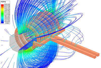
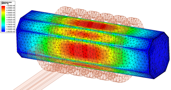
The streamlines of magnetic field intensity (ANSYS Maxwell). The eddy current loss on the surface of the cast iron rod (ANSYS Maxwell). The problem can also be solved with ANSYS Discovery AIM as shown in the following two figures.

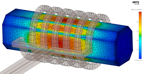
The magnetic field intensity in the cross-section of the problem (ANSYS Discovery AIM). The eddy current loss on the surface of the cast iron rod (ANSYS Discovery AIM).


References