Homework Assignment
|
Analysis of Shunt Resistor | ||
|
Instructor
|
Teaching Assistants:
| |
Aim of Assignment
Students will learn the basics of electromagnetic field calculations, their main steps, and gain practice in evaluating results and writing a Technical Report that meets international expectations.
Knowledge needed to solve the problem
- The main steps of the finite element method;
- Theoretical knowledge of the electromagnetic field simulation (for defining materials, for excitation);
- Knowledge of CAD system to create geometry;
- Download and install Ansys Electronics Desktop Student.
The Semester Assignment
The task consists of two parts, a basic task, with a faultless solution of up to 80%, and an extra task, with an additional maximum of 20%.
Deadline - Output Form: PDF format. Color drawings should be made so that their contents are clear to the reader in black and white. Language English Place of submission: In Moodle system. Late submission: After every day started, a 5% deduction from the achieved result (i.e. after 5 days delay 100% can only be obtained up to 100% - 5x5% = 75%). Evaluation: 0 - 48% - Insufficient [F] (1) 50 - 59% - Sufficient [D] (2) 60 - 70% Satisfactory [C] (3) 71 - 84% Good [B] (4) 85 - 100% - Very good [A] (5) For the formal requirements, the requirements of CFD and mechanics are also valid here.
Part I of the Assignment
Calculating the resistance and the total loss of the shunt resistor by finite element method
The geometry dimensions for your task you can find in the following table: Semester Assigment.
This task is a DC current conduction problem. The solved equation is
[math]\nabla\cdot\sigma\nabla \varphi=0[/math]
with following boundary conditions
[math]\vec{J}\cdot\vec{n}=-J_{\text{n}}[/math] on [math]\Gamma_{\text{J}}[/math] (This is the input.)
and
[math]\varphi=U_0 = \text{0 V}[/math] on [math]\Gamma_{\text{E}}[/math] (This is the output.),
where [math]J_{\text{n}}[/math] is the current density calculated from the specified current excitation.
The task: determine the voltage drop, the resistance and the ohmic loss of the problem.
The voltage drop is the potential difference between the two terminals of the arrangement. You can determine resistance using Ohm's law:[math]R = \frac{U}{I}[/math],
then the ohmic loss
[math]P = I^2\cdot R[/math]
where [math]U[/math] is the voltage drop, [math]I[/math] is the current and [math]R[/math] is the resistance.
Bulk conductivity of materials. Material Titanium Copper Aluminum Copper-manganin alloy [math]\sigma~[\text{MS/m}][/math] 1.82 58 38 20.833 Tasks
- Draw the geometry based on the specified dimensions in Ansys Electronics Desktop Student;
- Define the problem based on the given material parameters and boundary conditions;
- Run the FEM simulation;
- Evaluate the results.
The quantities listed in the task can be calculated with the Maxwell 3D - DC Conduction solver and the Q3D Extractor - DC solver.
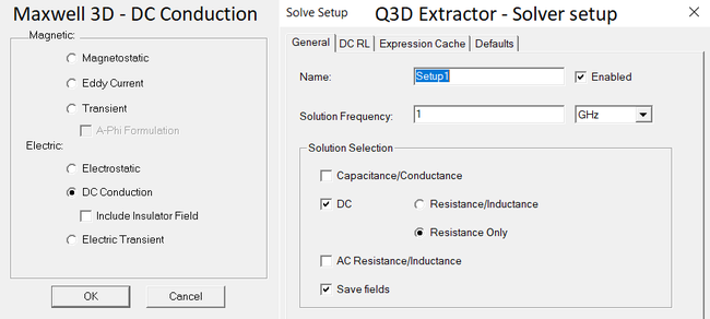
Figure 2. - Possible solution (Left - Maxwell 3D, Right - Q3D Extractor).
Results of the test example. Quantities Voltage drop [mV] Resistance [[math]\text{n}\Omega[/math]] Ohmic loss [W] Maxwell 3D 10.9927 18.3211 6.5956 Q3D Extractor 10.9759 18.2931 6.5855
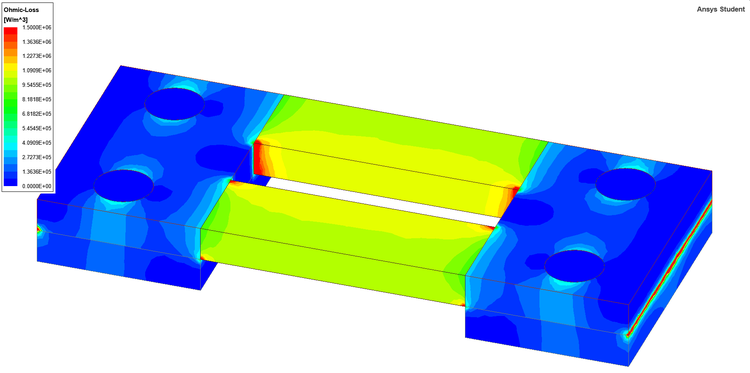
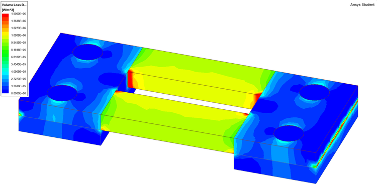
Ansys Maxwell 3D - Ohmic loss on the surface of shunt resistor. Ansys Q3D Extractor - Ohmic loss on the surface of shunt resistor. Step by step tutorials


Part II of the Assignment
In the student version of Ansys EM, Icepak provides an opportunity to study the thermal phenomena of the task. Ansys Icepak is a general CFD solver with specific capabilities for testing the heating and cooling of electronic circuits (PCB / power module).
The task has a natural convection cooling. The excitation is the ohmic loss from the electromagnetic simulation.
Thermal properties of materials. Material Titanium Copper Aluminum Copper-manganin alloy [math]\rho~[\text{kg}/\text{m}^3][/math] 4500 8933 2689 8400 [math]c_{\text{P}}~[\text{J}/(\text{kg}\cdot\text{°C})][/math] 522 385 951 410 [math]\lambda~[\text{W}/(\text{m}\cdot\text{°C})][/math] 21 400 237.5 22 The table below shows the result of the thermal simulation.
Results of the test example. Quantities Max. temperature [°C] Min. temperature [°C] Max. velocity [m/s] Maxwell 3D + Icepak 75.9284 71.3658 0.2881 Q3D Extractor + Icepak 75.8669 71.3002 0.2880

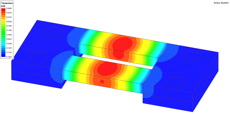
Ansys Maxwell 3D + Ansys Icepak - Temperature distribution on the surface of shunt resistor. Ansys Q3D Extractor + Ansys Icepak - Temperature distribution on the surface of shunt resistor. Step by step tutorials
Here you can find the archive file of test example: Shunt Resistor (Ansys EM Student 2021 R2).

