Lecture 2.

Basics of Finite Element Method / Time-Harmonic Magnetic Field
Instructor Dániel Marcsa (lecturer) Lectures: Monday, 14:50 - 16:25 (D201), 16:30 - 17:15 (D105) Office hours: by request	Teaching Assistants: - Office hours: -.

Finite Element Method (FEM)

Scalar finite element methods have been used by civil and mechanical engineers to analyze material and structural problems since the 1940s. However, it wasn't until the 1960s that FEM codes were developed to solve problems in electromagnetics. Some of the pioneers in this field were Silvester , Zienkiewicz, and Wexler. Initial FEM-based CEM modeling codes were applied to problems in electrostatics and magnetostatics. Later they were used to solve high-frequency problems in 2 dimensions. Practical 3-dimensional codes did not appear until the 1980s due largely to problems with vector parasites and unreliable absorbing boundary conditions. Unwanted reflections from absorbing boundaries continue to be a problem with full-wave 3D FEM codes even today.

Like BEM techniques, finite element methods can be based on different formulations (even the method of moments). However, BEM techniques always solve an integral equation and FEM techniques always solve a differential equation. Every FEM code divides the entire problem domain into small elements. For 2D problems, the elements are usually triangles or rectangles. For 3D problems, the elements are usually tetrahedra (4 faces) or bricks (6 faces). The domain must be finite and bounded. Modeling an unbounded (e.g. radiation) problem requires that the problem domain be bounded with special elements that absorb all incident energy. These elements are called ABC (Absorbing Boundary Condition) elements.

The unknowns in scalar FEM codes are the three orthogonal components of the field at the "nodes" (vertices) of each element. The unknowns in vector FEM codes are the field components along the edges of each element. Scalar codes are conceptually simpler, but they are unsuitable for full-wave modeling, because they are susceptible to spurious solutions that can cause significant and unpredictable errors in the solution. Vector FEM codes are much less likely to exhibit these parasitics.

To form a linear system of equations, the governing differential equation and associated boundary conditions are converted to an integro-differential form using either a variational method or a weighted-residual (moment) method. Variational methods solve for the unknown quantity by minimizing an energy functional. Weighted-residual methods multiply a weak form of Maxwell's equations by a weighting function and integrate over each element. Ultimately, a matrix equation is generated in the form,

[math]\textbf{A}\textbf{x}=\textbf{b}[/math]

where [math]\textbf{x}[/math] is a vector of the unknown field quantities, [math]\textbf{b}[/math] is a vector of source terms, and [math]\textbf{A}[/math] is a sparse matrix whose only non-zero values correspond to positions in the matrix corresponding to edges that share an element.

Generally, the matrices generated by FEM codes are must larger than the matrices generated by BEM codes applied to similar geometries. This is because gridding an entire problem volume requires many more elements than gridding just the material interfaces. However, because FEM matrices are very sparse, they do not necessarily require more storage or computing resources to solve than the small, but dense, matrices generated by BEM codes.

As indicated previously, modeling unbounded problems require special absorbing elements (ABCs). Many formulations of these elements have been proposed . The ABCs that have been developed for 2D FEM codes work very well; however, 3D FEM ABCs work well only at prescribed angles of incidence resulting in the need to locate the boundaries sufficiently far from other structures. Hybrid FEM/BEM codes terminate open surfaces of the FEM volume with a BEM surface negating the need for ABCs. Unfortunately, the BEM portion of the resulting matrix is dense, which can significantly increase the amount of computational resources required.

Perhaps the most attractive feature of the finite element method is its ability to model configurations that have complicated geometries and incorporate various materials. The electrical properties of each element are defined independently and elements can be as small or as large as needed to facilitate the analysis.

The following table summarize various strengths and weakness of FEM modeling techniques. Note that the capabilities of any particular modeling software depend on the specific formulation, the matrix solver and any optimization techniques employed.

Strengths	Weaknesses
Excels at modeling inhomogeneous or complex materials Excels at modeling problems that combine small detailed geometries with larger objects Excels at modeling structures in resonant cavities or waveguides	Absorbing boundary required for modeling unbounded (radiation) problems Difficult to model thin/electrically large or resonant wires accurately

Overview of time-harmonic equations and related problems

For time-harmonic fields, the time convention [math]e^{j\omega t}[/math] is used and suppressed and [math]\omega=2\pi\cdot f[/math] is angular frequency. Therefore, we can replace [math]\partial/\partial t[/math] by [math]j\omega[/math], and the differential form of Maxwell's equations reduced to

[math]\nabla\times\vec{H}=\vec{J}+j\omega\vec{D}[/math]	Maxwell-Ampére law,
[math]\nabla\times\vec{E}=-j\omega \vec{B}[/math]	Faraday's law,
[math]\nabla\cdot\vec{B}=0[/math]	Gauss's law (magnetic),
[math]\nabla\cdot\vec{D}=\rho[/math]	Gauss's law (electric),
[math]\nabla\cdot\vec{J}=-j\omega \rho[/math]	Current continuity equation.

The time-harmonic Maxwell's equations are employed for the steady state behaviour. The static case is the limiting case of time-harmonic fields as [math]\omega \to 0[/math]. The field quantities of time-harmonic Maxwell's equations are functions of position ([math]\vec{r}[/math]) only, and the phasor representation of fields has been employed. The relation between the phasor representation and its corresponding instantaneous version, with reference to [math]\cos(\omega t)[/math], is given by

[math]\vec{H}(x,y,z,t) = \Re\{\vec{H}(x,y,z)e^{j\omega t}\}[/math].

The use of time-harmonic fields is not as restrictive as it first appears. Using Fourier analysis, any time-varying field can be expressed in terms of time-harmonic components via the Fourier transform

[math]\vec{H}(t)=\int_{-\infty}^{\infty}\vec{H}(\omega)e^{j\omega t}\text{d}\omega[/math],

[math]\vec{H}(\omega)=\frac{1}{2\pi}\int_{-\infty}^{\infty}\vec{H}(t)e^{-j\omega t}\text{d}t[/math].

Therefore, if a time-harmonic field is known for any [math]\omega[/math], its counterpart in the time domain can be obtained by evaluating inverse Fourier transform.

Skin Depth

Skin depth or depth of penetration is an alternative way to characterize a medium with nonzero conductivity. It is defined as the distance measured from the surface of the lossy medium over which the magnitudes of the fields are reduced to [math]1/e[/math] or approximately 37%, of those at the surface of the medium. The skin depth [math]\delta[/math] of a good conductor ([math]\sigma/\omega\varepsilon \gg 1[/math]) is approximately given by

[math]\delta = \sqrt{\frac{2}{\omega\mu\sigma}}[/math].

The skin depth of a good conductor is very small, especially at high frequencies, causing currents to residue near the conductor's surface. The containment of current reduces the effective cross-section area of the conductor (increase the resistance) and therefore increases conduction loss.

Frequency [math][\text{Hz}][/math]	Loss [math][\text{W}][/math]	Resistance [math][\mu\Omega][/math]	Inductance [math][\mu\text{H}][/math]
50	0.12677	25.354	0.54144
500	0.32382	67.764	0.51372
5000	0.95942	191.88	0.50105
50000	2.9767	595.34	0.497

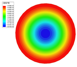
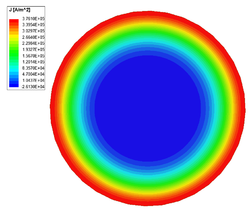
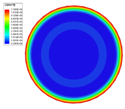
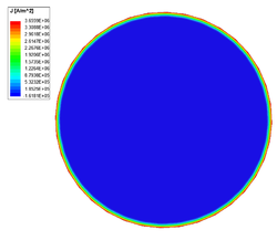
Current density in the cross-section of copper conductor at 50 Hz.	Current density in the cross-section of copper conductor at 500 Hz.	Current density in the cross-section of copper conductor at 5000 Hz.	Current density in the cross-section of copper conductor at 50000 Hz.

References

- ↑ CVEL - https://cecas.clemson.edu/cvel/modeling/tutorials/techniques/fem/finite_element_method.html
- ↑ P. Silvester, "High-order finite element waveguide analysis (Program Descriptions)", IEEE Trans. on Microwave Theory and Tech., vol. 17, no. 8, pp. 651-652, Aug. 1969.
- ↑ 3.0 3.1 Y. Li and Z. Cendes, "High-accuracy absorbing boundary condition," IEEE Trans. on Magnetics, vol. 31, no. 3, pp. 1524-1529, May 1995.
- ↑ M. Kuczmann - Potential Formulations in Magnetics Applying the Finite Element Method, Lecture Note, University of Győr, 2009.