Lecture 3. - Assignment
|
Analysis of Permanent Magnet Motor | |
|
|
|
| Drive unit of Audi A3 Sportback e-tron drivetrain.[1] | Operation of a permanent magnet synchronous motor. [Click to see animation.] |
|
Instructor
|
Teaching Assistants:
|


Contents
Purpose of the Assignment
The student will learn the main steps of the finite element method, such as preparing the model (creating or importing geometry), specifying material parameters, boundary conditions, and excitation through a time-dependent simulation. Promote understanding of the source of unwanted phenomena of rotating electrical machines, like noise, vibration and heat.
Knowledge needed to solve the problem
- The steps of the finite element method;
- Theoretical knowledge of time-varying magnetic fields (for defining materials, excitation);
- Basic knowledge of electrical machine operation.
Steps to solve the problem
After launching ANSYS Electronics Desktop, open the file PM_Motor_Example.aedt using the File [math] \to [/math] Open menu.
To use ANSYS Maxwell, the Help menu and YouTube videos provide a lot of help.
Defining the Problem
In this case, the geometry and definitions/settings of the problem are pre-defined. The reason for this is to avoid lengthy setup and basically, the purpose of the example is to look at sources of unwanted phenomena (force, loss) as an example of a rotating electric machine.
Before and during the run, we briefly review the settings of the problem.
It is important to note that in the previous two examples, adaptive meshing used. However, in the case of a time-dependent (transient) problem, it is not possible to use the adaptive mesh, so we need to define the discretization of the problem with different mesh operations.

Set up the solver, run the simulation
At the solver, the end of the time interval of calculation should be defined as well as the time step. In this example, the end time is 15 ms (Stop time) and 0.05 ms (100 time steps per period) is the time step.
You may also need to set the nonlinear solver, because the [math] {B} - {H} [/math] relation of the stator and rotor steel is nonlinear. In this case, the relative permeability is space dependent, as you can see in Fig. 1.
In order to plot the result at several time instants, it is necessary to specify in which time step we want to save the solution. If we do not do this, the last time step is saved automatically, so the field quantities ([math]\vec{A}; \vec{B}; \vec{H}[/math]; ...) or other derived quantities ([math] \text{loss}, \text{energy}, ... [/math]) can be plot in this instance.
Evaluation of results
The purpose of this example is to illustrate the source of undesirable phenomena in electric machines. The source of the heat is the loss in the various parts of the machine. We have already met with the eddy current loss in the previous lecture. However, the so-called electric steels has more components for core loss
- [math] p_{\text{vas}} = p_{\text{h}} + p_{\text{c}} + p_{\text{e}} = K_{\text{h}}f(B_{\text{max}})^2 + K_{\text{c}}(f B_{\text{max}})^2 + K_{\text{e}}(f B_{\text{max}})^{1.5} [/math],
where [math]p_{\text{h}}[/math] is the hysteresis loss, [math]p_{\text{c}}[/math] is the eddy current loss, [math]p_{\text{e}}[/math] is the excess loss, [math]K_{\text{h}}, K_{\text{c}}, K_{\text{e}}[/math] is the coefficient of losses, [math]f[/math] is the frequency and [math]B_{\text{m}}[/math] is the maximum of magnetic flux density. Fig. 1 shows the core loss and its components as a function of time.
The other main undesirable phenomenon is the vibration of electric machines. Here, we only deal with the main electromagnetic source of the vibration, the air-gap flux density, which differs from pure sinus, so it has harmonic content (harmonic content hardly depend on the design of machine). According to the Maxwell stress tensor, the tensile force (radial force magnitude) acting on the stator and on the rotor surface is proportional to the square of the normal component of the air-gap flux density. The Maxwell stress tensor can be calculated with the following relationship
- [math]\vec{\sigma} = \frac{1}{\mu_0}\left(\vec{B}\cdot\vec{n}\right)\vec{B} - \frac{1}{2\mu_0}B^2\vec{n}[/math],
where [math]B = \|\vec{B}\|[/math] is the absolut value of magnetic flux density. Fig. 3 shows the force acting on the stator teeth.
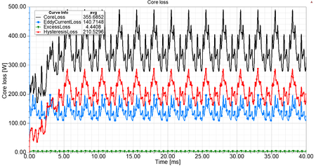
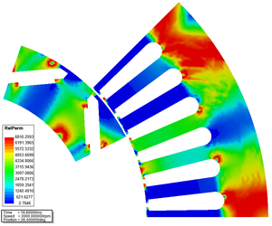
Fig. 1 - The core loss and its components in the function of time. Fig. 2 - The relative permeability in the stator and rotor core. Fig. 3 - The variation of teeth force as a function of time. [Click to see animation.]


