Lecture 4.

Integral Equations Based Methods / Wave Equations
Instructor Dániel Marcsa (lecturer) Lectures: Monday, 14:50 - 16:25 (D201), 16:30 - 17:15 (D105) Office hours: by request	Teaching Assistants: - Office hours: -.

Integral Equation Based Methods

Boundary Element Method (BEM)

Boundary Element Method (BEM) codes use the method of moments to solve an EFIE (Electric Field Integral Equation), MFIE (Magnetic Field Integral Equation) or CFIE (Combined Field Integral Equation) for electric and/or magnetic currents on the surfaces forming the interfaces between any two dissimilar materials. Most CEM modeling codes that bill themselves as simply "moment method" codes employ a boundary element method.

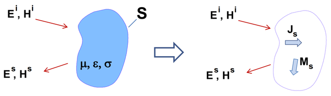
Figure 1. - Principle of Equivalence.

The first step in a boundary element analysis is to represent the problem geometry as a distribution of equivalent surface currents in a homogeneous medium (usually free space). As illustrated in Figure 1, the fields exterior to an object consist of fields incident on the object, fields reflected from the object and fields emanating from the object. The Equivalence Theorem states that any field distribution exterior to an object can be exactly duplicated by removing the object and replacing it with a set of equivalent electric and magnetic currents on the boundary surface.

Since the forms of EFIE and MFIE used by boundary element methods are only valid for current distributions in a uniform homogeneous medium, all objects in the problem space must be removed and replaced with (initially unknown) surface currents conforming to their boundaries.

Equations below show a common form of the EFIE and MFIE employed by boundary element method codes that model metallic objects only (i.e. there are no equivalent magnetic surface currents);

[math]\vec{E}(\vec{r})=\frac{-j\eta}{4\pi k}\int_S\vec{J}_S(\vec{r}')\cdot\vec{G}_e(\vec{r},\vec{r}')\text{d}S'[/math];

[math]\vec{H}(\vec{r})=\frac{1}{4\pi}\int_S\vec{J}_S(\vec{r}')\times\nabla'\vec{G}_m(\vec{r},\vec{r}')\text{d}S'[/math].

In these equations, [math]\int_S \text{d}S'[/math] integral over the surface represents integration over all boundary surfaces. Note that since the boundary only exists at places where an interface between two different materials occurred, the size of the boundary is limited (i.e. there is no integration to infinity).

The functions [math]\vec{G}_e[/math] and [math]\vec{G}_m[/math] in these equations relate source currents to the electric and magnetic field generated by those currents, respectively. [math]\vec{G}_e[/math] and [math]\vec{G}_m[/math] are called Green's functions and they play a central role in boundary element analysis. Free-space Green's functions express the field emanating from the surface current represented by an individual basis function (e.g. the current on an individual surface patch). However, other Green's functions can be employed to express the field emanating from more complex structures that are common to a particular problem geometry. For example, a geometry consisting of metal surfaces coated with a thin dielectric may employ a special Green's function that expresses the fields emanating from the combined surfaces of the metal-dielectric and dielectric-air interfaces. This can substantially reduce the number of surface elements required to model the problem.

All Green's functions are approximate expressions that are accurate for a limited range of frequencies, distances and source geometries. Many boundary element methods employ several Green's functions to model different regions of a problem or different problem environments.

General purpose 3D BEM codes usually employ basis and weighting functions that are linear current distributions on a rectangular or triangular surface patch. There are generally two unknowns per patch corresponding to two orthogonal current vectors. Thin wires can be represented very efficiently with a single unknown representing the amplitude of the current distribution on each wire segment.

Point matching techniques employ basis and weighting functions that are simple impulse functions often at the center of each patch or segment. Pulse matching techniques employ basis and weighting functions that have a constant value everywhere on the patch or segment. More accurate implementations employ basis and weighting functions that transition smoothly from one patch to the next. Rao-Wilton-Glisson (RWG) basis functions are a popular choice for codes that employ triangular surface patch elements. Roof-top basis functions are often employed by codes that use rectangular elements.

Generally, CEM software employing a boundary element method excels at modeling unbounded problems, particularly when it is not necessary to model regions of great complexity in detail. Structures that can be adequately represented with a wire grid can be analyzed very effectively using boundary element methods, because these methods model wires very efficiently.

Following table lists various strengths and weakness of BEM modeling techniques. Note that the capabilities of any particular modeling software depend strongly on the form of the integral equation solved, the choice of basis and weighting functions, the Green's function(s) employed, and the matrix solver and any optimization techniques employed.

Strengths	Weaknesses
Excellent for modeling unbounded (radiation) problems. Excellent for modeling metal plates and thin wires. Good for modeling structures with lumped circuit elements included.	Does not model inhomogeneous or complex materials well. Not good for modeling problems that combine small detailed geometries with larger objects. CFIE formulation required to model enclosed structures of resonant size.

Method of Moments (MoM)

In the 1960s, R.F. Harrington and others applied a technique called the Method of Moments to the solution of electromagnetic field problems. The Method of Moments (also called the Method of Weighted Residuals) is a technique for solving linear equations of the form,

[math]\mathcal{L}(\phi)=f[/math]

where the functional [math]\mathcal{L}(\bullet)[/math] is a linear operator, [math]f[/math] is a known excitation or forcing function, and [math]\phi[/math] is an unknown quantity. To solve this problem on a digital computer, we start by expressing the unknown solution as a series of basis or expansion functions, [math]v_n[/math],

[math]\phi = \sum_{n=1}^{N}a_n v_n[/math]

where [math]a_n[/math] are unknown coefficients describing the amplitude of each term in the series.

Now instead of one equation with a continuous unknown quantity, [math]\phi[/math], we have an equation with [math]N[/math] scalar unknowns,

[math]\mathcal{L}(a_1v_1+a_2v_2+\dots+a_Nv_N)=f[/math].

To solve for the values of [math]a_n[/math], we need [math]N[/math] linearly independent equations; so [math]a_n[/math] different weighting or testing functions, [math]w_n[/math], are applied. This yields the following system of [math]N[/math] equations in [math]N[/math] unknowns:

[math] \begin{bmatrix} \langle w_1,\mathcal{L}(v_1)\rangle & \langle w_1,\mathcal{L}(v_2)\rangle & \cdots & \langle w_1,\mathcal{L}(v_N)\rangle \\ \langle w_2,\mathcal{L}(v_1)\rangle & \langle w_2,\mathcal{L}(v_2)\rangle & \cdots & \langle w_2,\mathcal{L}(v_N)\rangle \\ \vdots & \ddots & \vdots \\ \langle w_N,\mathcal{L}(v_1)\rangle & \langle w_N,\mathcal{L}(v_2)\rangle & \cdots & \langle w_N,\mathcal{L}(v_N)\rangle \end{bmatrix} \begin{bmatrix} a_1 \\ a_2 \\ \vdots \\ a_N \end{bmatrix} = \begin{bmatrix} \langle w_1, f_1 \rangle \\ \langle w_2, f_2 \rangle \\ \vdots \\ \langle w_N, f_N \rangle \end{bmatrix} [/math]

This linear system of equations has the form,

[math]\textbf{A}\textbf{x}=\textbf{b}[/math]

where the elements of [math]\textbf{A}[/math] are known quantities that can be calculated from the linear operator, the functional [math]\mathcal{L}(\bullet)[/math], and the chosen basis and weighting functions. The elements of \textbf{b} are determined by applying the weighting functions to the known forcing function. The unknown elements of [math]\textbf{x}[/math] can be found by solving the matrix equation. After solving for [math]\textbf{x}[/math] (i.e. the unknown coefficients, [math]a_n[/math]), the value of [math]\phi[/math] is determined using [math]\phi = \sum_{n=1}^{N}a_n v_n[/math] equation.

The Method of Moments (MoM) can be used to solve a wide range of equations involving linear operations including integral and differential equations. This numerical technique has many applications other than electromagnetic modeling; however the MoM is widely used to solve equations derived from Maxwell's equations. In general, moment method codes generate and solve large, dense matrix equations and most of the computational resources required are devoted to filling and solving this matrix equation. The particular form of the equations that is solved and the choice of basis and weighting functions have a great impact on the size of this matrix and ultimately the suitability of a given moment method code to model a given geometry.

Equation Options

The most common equation form solved by CEM modeling codes based on the Method of Moments is the Electric Field Integral Equation (EFIE). This is an equation of the form,

[math]\vec{E}=f_e(\vec{J},\vec{M})[/math],

where [math]\vec{E}[/math] is the impressed (i.e. source) electric field and [math]\vec{J}[/math] and [math]\vec{M}[/math] are the induced electric and magnetic current densities, respectively. The EFIE will be discussed further in the section describing the Boundary Element Method. Generally, codes that solve a form of the EFIE excel at modeling open (unbounded) geometries in which the electric field dominates in the near-field region of the source.

Another equation solved by Moment Method codes is the Magnetic Field Integral Equation (MFIE), which has the general form,

[math]\vec{H}=f_m(\vec{J},\vec{M})[/math],

where [math]\vec{H}[/math] is the impressed (i.e. source) magnetic field intensity. Codes that solve a form of the MFIE are best suited for modeling geometries with circulating currents, where the magnetic near field is dominant.

Moment Method codes based on the EFIE or MFIE alone, may exhibit unstable behavior when the modeling surfaces form a resonant cavity at a particular frequency. To avoid this, many moment method codes solve a linear combination of the EFIE and MFIE known as a Combined Field Integral Equation (CFIE). This requires more calculations to fill the matrix, but results in a more stable solution when the modeling surface is large enough to support an interior resonance.

Some CEM modeling codes employ the Method of Moments to solve other equations. For example, static modeling codes often solve a form of Laplace's equation relating electric field strengths to charge densities or magnetic field strengths to current densities. The Generalized Multipole Technique (GMT) employs a moment method to solve equations for the electric field generated by multipole sources.

Basis and Weighting Function

An appropriate choice of basis and weighting functions can make a tremendous difference in the number of elements, [math]N[/math], required to obtain an accurate solution. Since the solution is represented as a summation of basis functions, it is important to choose basis functions that accurately represent the solution with a small number of terms. For example, when solving for the current distribution on a surface, the basis functions should be current distribution elements that can be summed together in a way that is able to efficiently approximate any overall current distribution that might result from the analysis.

Weighting functions should be chosen that maximize the linear independence of the various weighted forms of the equation. Often, the best choices of weighting functions are functions that are identical to the basis functions. Moment method techniques that employ identical basis and weighting functions are called Galerkin techniques.

Wave Equations

We will deal with the time-harmonic case directly in terms of the electric and magnetic fields. For this, it is necessary to derive from Maxwell's equations, which involve both electric and magnetic fields, the governing differential equations involving only either field.

Vector Wave Equations

The differential equation for [math]\vec{E}[/math] can be obtained by eliminating [math]\vec{H}[/math] from time-harmonic Faraday's law and time-harmonic Maxwell-Ampére law with the aid of the constitutive relations. Doing this, one obtains

[math]\nabla\times\left(\frac{1}{\mu}\nabla\times\vec{E}\right)-\omega^{2}\varepsilon\vec{E}=-j\omega\vec{J}[/math].

Similarly, one can eliminate [math]\vec{E}[/math] to find the equation for [math]\vec{H}[/math] as

[math]\nabla\times\left(\frac{1}{\varepsilon}\nabla\times\vec{H}\right)-\omega^{2}\mu\vec{H}=\nabla\times\left(\frac{1}{\varepsilon}\vec{J}\right)[/math].

These equations are called inhomogenoius vector wave equations. It is evident that the solution of [math]\vec{E}[/math] field also satisfies magnetic Gauss's law, and the solution of [math]\vec{H}[/math] field also satisfies electric Gauss's law.